"Bollinger Band mean reversion can win if you find the right settings."

If you still believe that, I won't mince words: stop reading this page and quit FX right now.

I slammed "10,000 combinations" of parameters against EURUSD market data from 2005 to 2025—25 years of history. Hundreds of billions of calculations. After pushing the limits of physical computation, the conclusion is singular:

There is not a single shred of a "Holy Grail" in Bollinger Band mean reversion.

Thin maxims like "You'll win with a high risk-reward" or "It's theoretically profitable if RR is over 1" have been reduced to pathetic rubble before the weight of 25 years and the judgment of statistics.

In this article, I will expose the results of Bollinger Band testing that I burned out my CPU to uncover.

The Scope of This Verification

In this study, we will investigate whether Bollinger Band mean reversion actually works.
The method is Brute Force Verification.

Simply put: entry occurs when price action hits the BB mean reversion criteria, and exit occurs at specified Take Profit (TP) and Stop Loss (SL) pips.
It is incredibly simple, but this is the most fundamental approach—the same philosophy that brings profits to elite hedge funds.

"We saw that there were some anomalies in the data that we could exploit." —— Jim Simons (Founder of Renaissance Technologies) quoted from his TED Interview

"Investment is a scientific process, continuing to verify thousands of hypotheses through rigorous data analysis." —— Two Sigma (from the official report: The Innovation Equation)

First, Testing with Common Settings

Let's look at how the verification is actually performed.
Below is the screen of the free backtesting tool, Delver.

Test Object

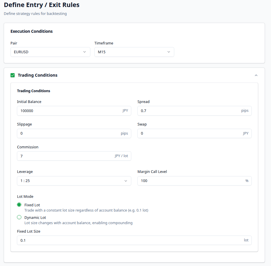
• Symbol/Timeframe: EURUSD 15-Minute (M15)
• Spread: 0.7 pips
• Slippage and Swap: Disabled
• Leverage: 25x
• Risk Management: Fixed Lot (Since this is a test of the strategy, not fund management)

Bollinger Band Settings

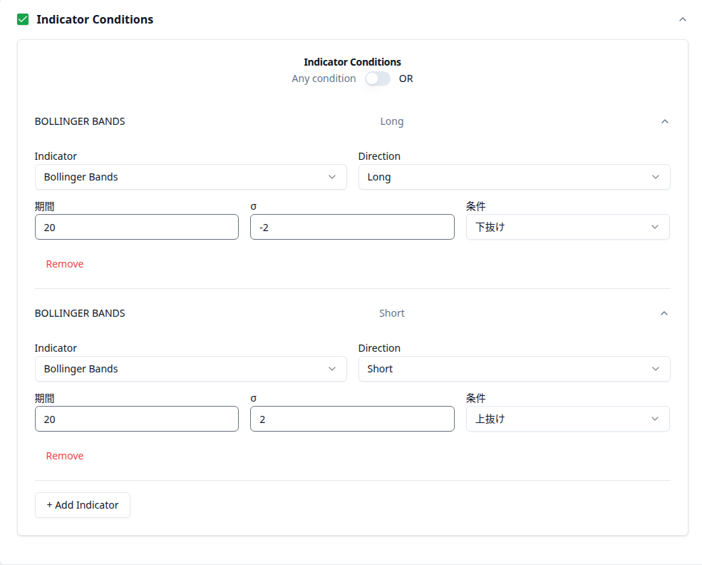
A basic setup entering at 2 or -2σ. The period is the standard 20.

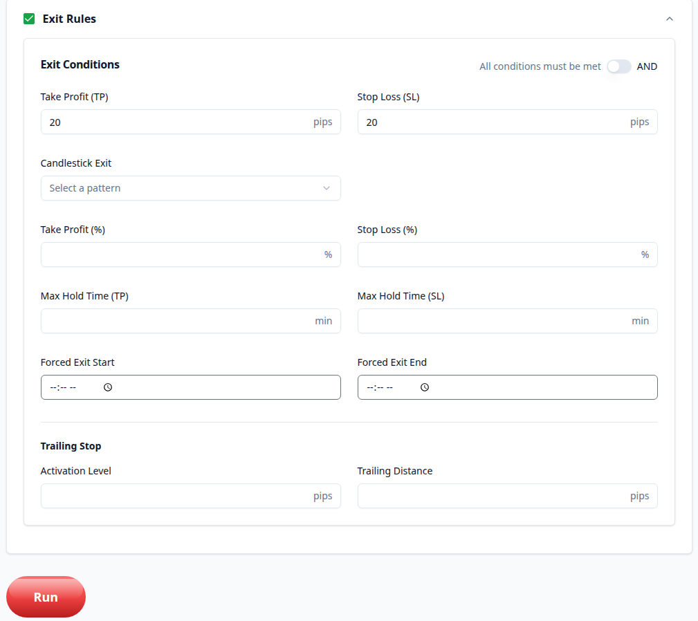
This is also a standard RR1 Exit setup.
Some might argue that results change based on TP and SL, but I will address that later.

Verification Results

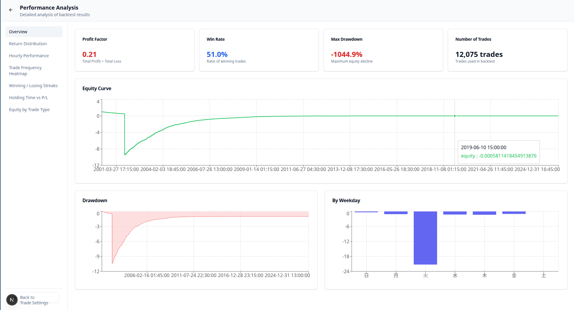
The results were catastrophic, leading to a total wipeout of the account.

• Profit Factor 0.21: This doesn't even qualify as an investment. It means you are losing 5 times the amount you earn.
• Max Drawdown -1044.9%: Your account wouldn't just be blown; it would need to be blown 10 times over to cover the loss.
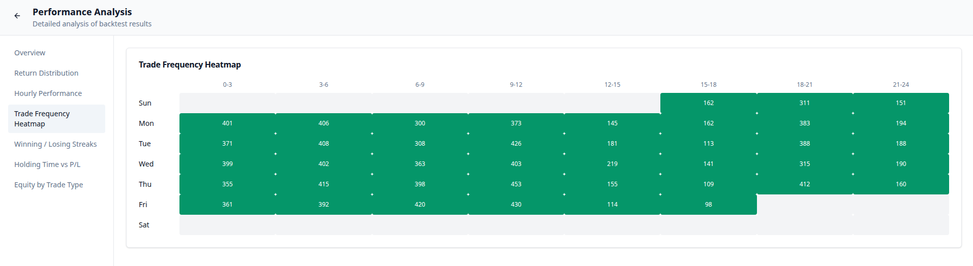
• Performance by Day: Tuesday alone showed devastating losses (approx. -21.0). It's clear that this isn't something that can be saved by avoiding specific days or times.
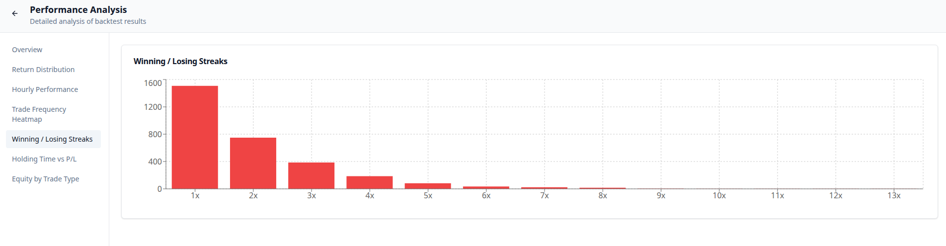
• Losing Streak: A record of 13 consecutive losses. If you were to believe in Bollinger Band "mean reversion" and try to Martingale/Average down, you would be led to ruin in an instant.

These are miserable results, but this is only one test.
It would be premature to think you understand everything from this alone.
You might be curve-fitting, so it’s dangerous to assume you’ve actually verified anything yet.
Let’s take a much deeper look.

The Hypothesis: "It Depends on the Exit Condition"

In the previous test, both were fixed at 20 pips. Was that the problem?
Since the timeframe is short, should we shorten the profit line to increase the win rate?
Or would the Profit Factor increase if we followed the "Cut losses short, let profits run" mantra?
Numerous hypotheses arise.
In the next section, let’s test all of these hypotheses at once.

Brute Force Verification with Python

While I could have used Delver, I decided to run this through Python as it involves over 10,000 combinations.

Overview of the Verification

• Entry Condition: Mean reversion entry on Bollinger Band 2, -2σ touch
• Take Profit (TP): 5 to 100 pips (1 pip increments)
• Stop Loss (SL): 5 to 100 pips (1 pip increments)
• Verification Period: 5 years (EURUSD M15, 2020 to 2025)
• Total Trades: Simulations spanning millions of trades
• Etc: Spread and risk conditions are identical to the Delver setup above

With this setup, I will perform a brute force test in 1-pip increments—testing everything from "TP 5 / SL 10" for high win rates to every other possibility.
By doing this, the bias during verification regarding exits is eliminated.

Verification Results

The verification results were startling.

Expectancy

Below is a histogram showing the distribution of expectancy.

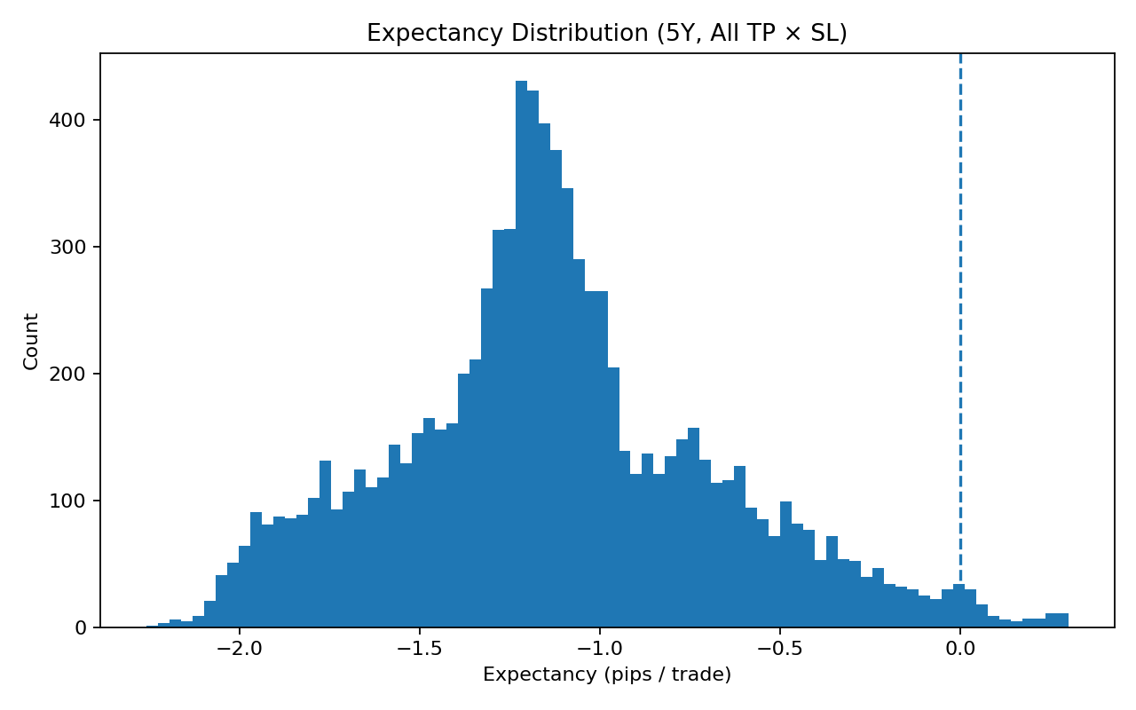
While the vast majority of expectancy is negative, there is a small minority that is positive, which seems promising.

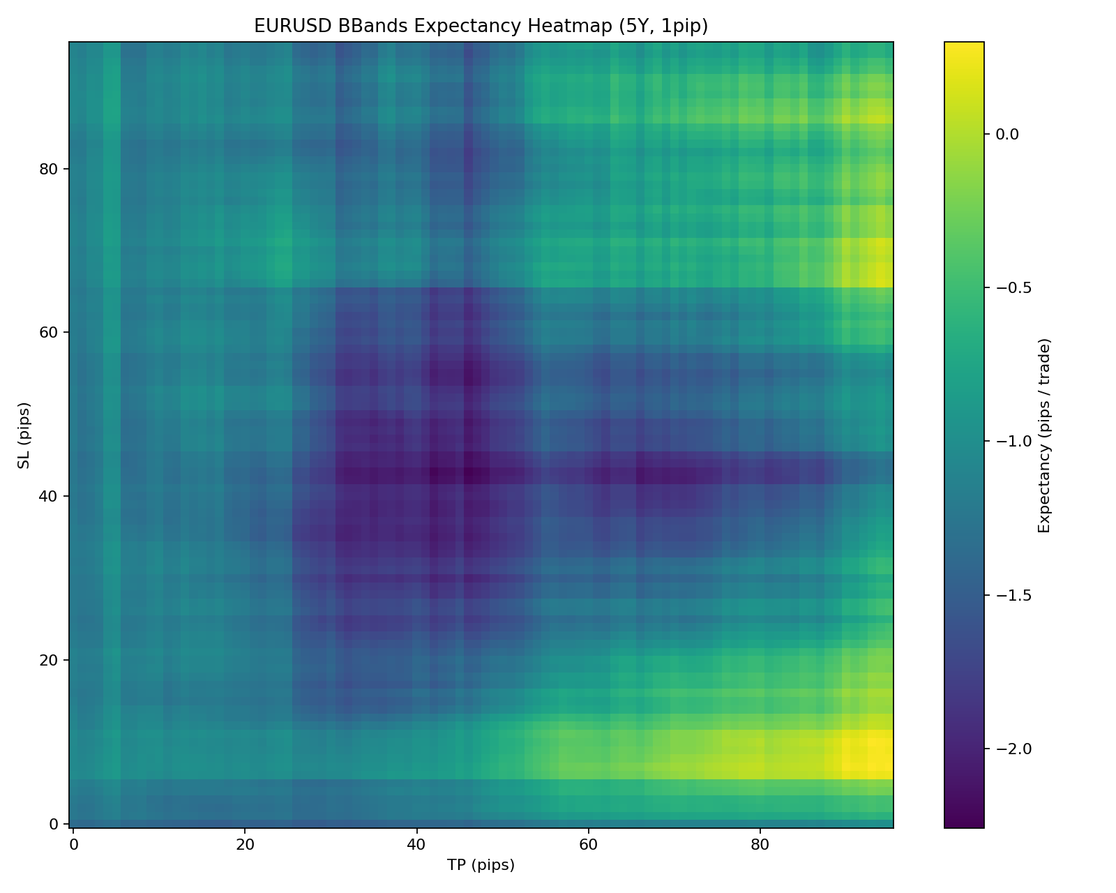
This is a heatmap representing the relationship between TP, SL, and expectancy.
As you can see, the vast majority of the heatmap is stained with blue and purple—the colors of death.
However, there are spots glowing in yellow, indicating positive expectancy.

"If I extend profits and place stop losses appropriately, Bollinger Band mean reversion can be profitable—."
For a moment, I held onto hope as I found this "Golden Area" at the end of exhaustive calculations.

But do not be deceived.

As an engineer, I decided to subject this "Golden Area" to two even more brutal and persistent tests to see if it was the real deal.

Visualizing Drawdown

Drawdown is one of the most critical elements in verification.
Even with a high win rate, I have personally experienced many times how the curse of drawdown can result in repeated losses.
Many traders have felt this.
However, look at the heatmap below:

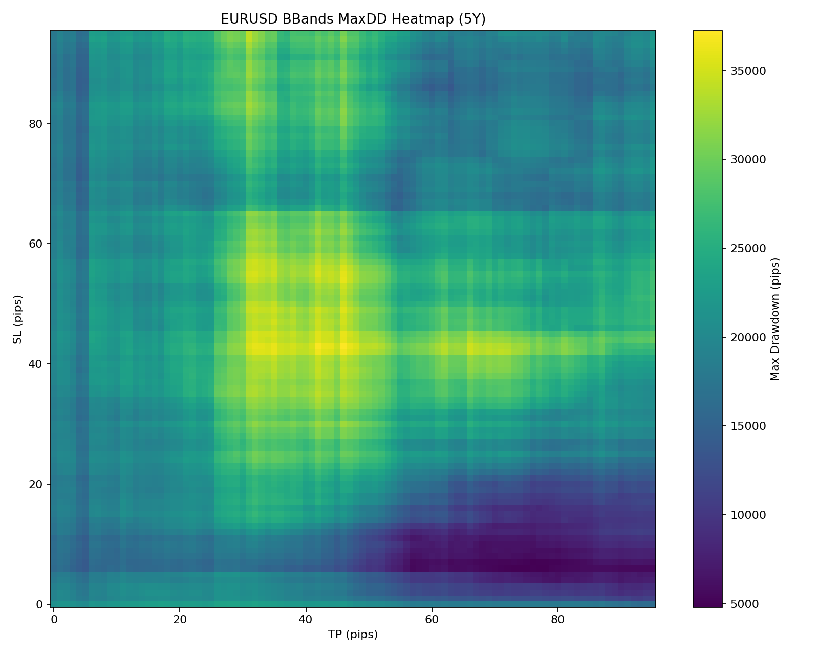
The reading of this map is simple:

• Yellow Area: The "Dead Zone" where drawdown is extremely high.
• Blue Area: The "Safe Zone" where drawdown is kept low.

Now, look at the expectancy heatmap below one more time.

In the bottom right of the map, where the expectancy glowed brightest... do you see the "Blue Spots" where drawdown is suppressed?

"Profits (expectancy) are maximized, and risk (drawdown) is minimized."

At the end of the madness of 10,000 brute force tests, I might have finally grasped the mathematically backed "True Holy Grail."

If I trade with this combination, is it perhaps impossible to lose? With trembling hands, I threw this "Golden Setting" into an even more grueling 25-year endurance test.

Verifying 25 Years with Only the Elite Conditions

Based on the previous results, Bollinger Bands seemed like an incredibly promising indicator.
So, I tested whether trading under the high-expectancy, low-DD conditions I defined would truly result in a positive outcome over 25 years of data.

Defining "Elite Conditions"

As explained in the previous graphs, I wanted to extract the overlapping blue and yellow areas from the heatmaps. Let's define this more precisely.

Below is a brief explanation of the Python logic used to define these elite conditions:

Trade Count Filter

df = df[df["trades"] >= MIN_TRADES_5Y]

This extracts only conditions with more than 400 trades over 5 years. The reason is to exclude curve-fitting—where someone just got lucky with a few trades—and to ensure the statistical stability of the expectancy. This removes individuals without reproducibility.

Max DD Filter

df = df[df["max_dd"] <= MAX_DD_PIPS_5Y]

This extracts individuals with a maximum DD of 5,000 pips or less over 5 years, eliminating those that would be bankrupt from a fund management perspective. For example, even if a setup had a Profit Factor over 1 until 2008, it's useless in practice if the DD became too deep after 2009.

Normalizing DD by Trade Count

dd_per_trade = df["max_dd"] / df["trades"]

Due to spreads, strategies with more trades tend to have higher cumulative DD. To ensure fairness across different frequencies, I applied this measure since our focus is on whether Bollinger Bands can win.

Score Calculation

score = Expectancy - 0.30 × (Max DD / Trades)

I decided to evaluate individuals using a score centered on expectancy. In other words, strategies with large DD are penalized, while those with small DD are highly rated if the expectancy is the same.

And here is the result of adopting only the top-scoring elite conditions:

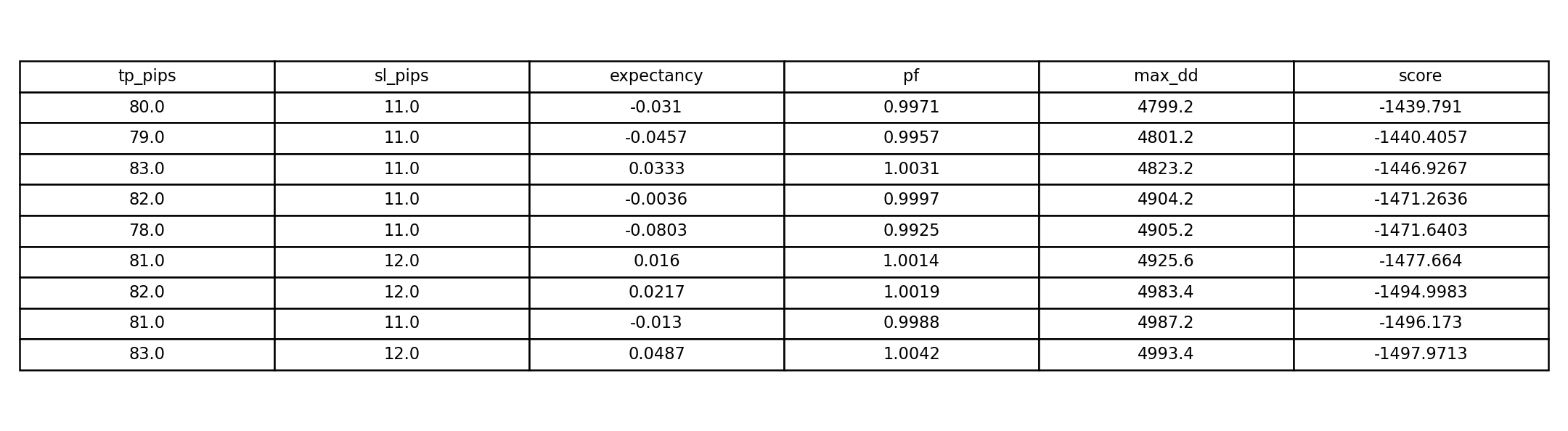
Results of the Elite Conditions

Rather than explaining, I'll let the resulting graph speak for itself.

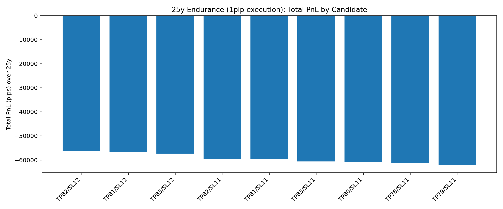
In this graph, the vertical axis represents PnL (Profit and Loss) and the horizontal axis represents the exit conditions.
It goes without saying: every single one is negative. A total wipeout.

However, it is a bit nonsensical to conclude simply that Bollinger Bands are "useless" based only on this. Let's analyze.

Why did the previously "Elite" conditions turn negative?

This graph exposes the essence of trading and verification.

Cumulative Losses from Spreads

Over 5 years, the 0.7 pip round-trip didn't impact the DD as much, but over 25 years, the cumulative loss from spreads becomes monumental.
Since the timeframe was M15 and the Stop Loss was as tight as 11 pips, it’s clear the entry frequency was scalping-like. The strategy fell victim to the inherent weakness of scalping—cumulative costs leading to massive losses.

It was just "Lucky" timing.

Five years might seem like a sufficient period, but when viewed across a 25-year span, it was merely a fragment of time.
However, I believe it is more productive to assume this: Bollinger Bands had an edge between 2020 and 2025. This is the greatest takeaway of this verification.

Summary

Let's summarize what we've learned from this study:

• Bollinger Bands only function under extremely limited conditions.
• Trading Bollinger Bands in isolation causes expectancy to converge to negative in the long run.
• The cumulative effect of transaction costs (spreads) becomes fatal over long periods.

These are the facts. However, the important part starts here.

Bollinger Bands are not "Useless"

We were able to discover specific periods where expectancy was positive. Just because 99% of settings have negative expectancy doesn't mean we should jump to the conclusion that Bollinger Bands are useless. That is too short-sighted.
However, it is a fact that if you continue to trade Bollinger Bands alone, you will be in a structure where your capital is slowly ground away.

Identifying when the Bollinger Band Edge exists.

This is the most important part of this article.
Namely: "Verification exists to find the Edge."

In this study, we were able to roughly grasp the timing when Bollinger Bands have an edge.
Now, we can:

• Filter by day of the week
• Use longer timeframes
• Filter by Price Action
• Filter by Trend

The list is endless, but extracting that edge is the essence of verification.

This kind of verification doesn't necessarily require Python. There are many completely free verification tools available.
The verification tool used this time, Delver, is exceptionally compatible with this kind of brute force testing. However, it's best to choose a verification tool that fits your trading philosophy, so I recommend comparing them for your own research.

Open Source Research

To ensure transparency and reproducibility, I have open-sourced the Python scripts used for this extensive backtest. You can review the logic behind the data processing and the statistical calculations on GitHub.

👉 Trade Verification Bollinger Bands Research